Rambling about Statistics using the FIFA WC as an Excuse
The FIFA World Cup is right around the corner. Hosted jointly by the United States, Canada and Mexico, this is the most structurally different tournament in a generation.
The competition has expanded to 48 teams divided into 12 groups of four, introducing a completely new dynamic to qualification, squad rotation, and knockout progression.
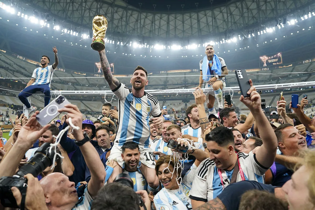 In this blog, I will attempt to analyze the favourites for the WC, and try to predict a winner for the tournament.
Analytics 101
Before I begin dissecting the teams and try to predict a winner, I would first like to give a small crash course on some common terminologies used in football analytics.
Expected Goals (xG)
xG is the foundational metric of modern football analytics, and something that you will encounter everywhere. It tells us how likely a player is to score a goal from a chance. The idea of xG is simple: not all shots are created equal. A tap-in from 2 yards, and a free kick from 30 yards out are both shots, but they both obviously have wildly different probabilities of the ball hitting the back of the net. xG tells us the quality of the shot taken. The simplest method to model xG would be with Logistic Regression: $$P(Goal) = \frac{1}{1+e^{-(\beta _ 0 + \beta_1x_1 + \beta_2x_x + ... + + \beta_nx_n )}}$$ Common factors here can be things such as, but not limited to, shot distance, angle to goal, presence of defenders, and so on.
Interpreting xG
Interpreting xG is rather simple: if a chance has an xG of 0.2, it means that based on historical observations, the possibility of the goal going in is 20%. Cumulative xG over all the chances presented to a team can be used as a metric to find the underlying attacking strength of your team. For example, a team that scores 4 goals from 1.2 xG in a game, can be assumed that it is performing well beyond expectations. And another team, that scores 2 from 3.8 xG, can be said that they got unlucky, or performed below their expected level
Expected Goals Against (xGA)
xGA is a the same metric as xG, but from the defensive side. It helps us find which teams are defending better than expected, and which teams are struggling in their defence.
Note: There is a lot of xG yap (as it is the most commonly used metric in football analytics), but sadly due to lack of data for many teams in the games leading up to the World Cup, I could not use the standard xG and xGA metrics in the models below. Teams can change significantly between multiple tournaments, and it just did not feel right to solely depend on metrics from the last set of major international tournaments, which were held in 2022 and 2024.
Elo Ratings
Elo is a rating system that is used for zero-sum games. A Zero-sum game describes any competitive interaction where one party's gain is offset by another party's loss. The name 'Zero sum' comes from the mathematics behind it: if you sum all gains and losses across every participant, the result is always zero. This applies cleanly to any head-to-head competition, including football. Every game produces exactly one result, and whatever one side gains fro that result, the other side forfeits by the same amount. Rating points can only move between teams, and the total supply is fixed. Over time, this rating becomes a good measure of a team's performance. A high rating implies that a team has consistently beaten strong opponents.
The Elo system was initially built by Arpad Elo, a Hungarian-American mathematician and a Chess player. Elo's central assumption was that the chess performance of each player in each game is a normally distributed random variable. Even if a player may perform significantly better or worse from one game to the next, the mean value of the player's performance changes slowly, highlighting a general trend of performances, instead of judging a player solely by a freak result. This makes an Elo system a self-correcting system.
If two players A and B have ratings $R_a$ and $R_b$, the expected scores of the players are $E_A = \frac{1}{1+10^{(R_B - R_A)/400}}$ and $E_B = \frac{1}{1+10^{(R_A - R_B)/400}}$. A score of 1 represents a win, 0.5 a draw, and 0 a loss. If both teams are rated equally, $E_A=E_B=0.5$: the system treats it as a coin flip. A 200-point advantage pushes the stronger team's expected score to roughly 0.76. A 400-point gap puts it at around 0.91, and so on. The rating difference translates directly and continuously into a probability.
After the game, the players actually score $S_A$ and $S_B$, so their ratings are updated as:
$$R_A' = R_A + K(S_A - E_A) \quad \text{and} \quad R_B' = R_B + K(S_B - E_B)$$
where K is the maximum possible gain/loss per game. The bracket $(S_A - E_A)$ indicates the surprise element of the result. Beating a heavily inferior opponent is not surprising, and thus results in zero surprise. On the other hand, losing to a team well below you is a big upset, and you get penalized accordingly for losing to a weaker team.
FIFA adopted this Elo-based methodology in 2018, replacing a previous system that was widely criticized for rewarding teams that simply played more matches regardless of quality. FIFA's implementation adds one important layer on top of the base Elo formula: an importance coefficient I, which scales how many points are actually at stake in a given match (A friendly played outside an international window carries a coefficient of just 5, while a World Cup knockout match carries 60, 12 times the weight).
The full update formula is: $$P' = P+I(W−We)$$ where W is the actual result (1 for a win, 0.75 for a penalty shootout win, 0.5 for a draw or shootout loss, 0 for a defeat) and $W_e$ is the expected result, calculated as: $$W_e = \frac{1}{10^{-\Delta/600} + 1}$$ with $\Delta$ being the pre-match rating difference between the two sides. The scale factor here is 600 rather than the classical Elo value of 400.
An interesting observation: Adding up the Elo points of all the groups, we get the following chart:
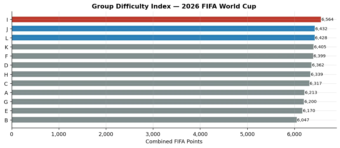 This year's edition sadly does not have any 'Group of Death', but the closest would be Group I, which has France (solid team, with multiple quality players), Norway (have Haaland and Odegaard), Senegal (AFCON 2026 Winners** atleast in my book) and Iraq.
On the other hand, Group B, consisting of Switzerland, Canada, Bosnia and Qatar is the group with the least quality, atleast by using elo as a metric.
The Dixon-Coles Model
To simulate a tournament meaningfully, predicting who wins each match is not enough. We need to predict how matches end. A team that wins 1–0 every game has a completely different tournament profile to a team that wins 4–2 every game. This sort of variance in scoring patterns determines how far a team can survive in a knockout tournament, where a single bad half can end everything, and where your bracket trajectory beyond the group stage depends entirely on where you finish in your group.
The Dixon-Coles model, introduced by Mark Dixon and Stuart Coles, addresses this directly. It is a statistical framework that models goals scored by each team as an independent Poisson random variable, incorporating team-specific parameters for attacking and defensive strength.
Goals as a Poisson Process
The model rests on a simple observation: goals are rare, discrete events that occur independently of each other, distributed unevenly over 90 minutes. A goal in the 23rd minute does not make a goal in the 67th minute more or less likely.
If a team scores an average of $\lambda$ goals per match (where $\lambda$ is the expected number of goals) given everything we know about the matchup, the probability of them scoring exactly $k$ goals is:
$$P(X = k) = \frac{e^{-\lambda} \lambda^k}{k!}$$
So if $\lambda = 1.4$, the probability of scoring 0 goals is $e^{-1.4} \approx 0.247$, exactly 1 goal is $0.346$, exactly 2 is $0.242$, and so on. Run this independently for both teams and you get a full probability distribution over every possible scoreline" 0–0, 1–0, 2–1, 3–2, and everything beyond. The question then becomes: how do we estimate $\lambda$ for a given team in a given match?
Attacking and Defensive Strength
Dixon and Coles model each team's expected goals as a product of three components:
$$\lambda_{H} = \alpha_H \times \beta_A \times \gamma$$
$$\lambda_{A} = \alpha_A \times \beta_H$$
Where $\alpha$ is the attacking strength of each team, $\beta$ is the defensive weakness of each team, and $\gamma$ is a home advantage multiplier. For the World Cup, which is played at neutral venues, $\gamma = 1$ for all teams except a small upward adjustment for the three host nations (USA, Canada, and Mexico).
The original paper estimates $\alpha$ and $\beta$ via maximum likelihood estimation across historical match data, which involves an optimisation procedure that is statistically rigorous but somewhat opaque. Fortunately, we have xG now. We can estimate these parameters directly and transparently from FBref data:
$$\alpha_{team} = \frac{\text{xG per 90 (last 20 matches)}}{\text{avg xG per 90 across all teams}}$$
$$\beta_{team} = \frac{\text{xGA per 90 (last 20 matches)}}{\text{avg xGA per 90 across all teams}}$$
Both values are centered on 1.0: A team with $\alpha = 1.3$ generates 30% more expected goals than the average international side, and a team with $\beta = 0.7$ concedes 30% fewer. To convert these relative strength ratios into an actual expected goals figure, we anchor them to $\bar{\lambda}$, the baseline average rate of goals in international football (approximately 1.3 goals per team per match):
$$\lambda_{A} = \alpha_A \times \beta_B \times \bar{\lambda}$$
This is the number that feeds directly into the Poisson formula. Team A's attacking strength, scaled by how weak team B's defence is, scaled by what the average actually means in goals. Without $\bar{\lambda}$, $\alpha \times \beta$ is a dimensionless ratio. With it, you get an expected goals figure you can simulate from.
The Low-Score Correction
A pure independent Poisson model has one well-documented flaw: it underestimates the frequency of low-scoring matches. Empirically, 0–0 draws, 1–0 wins, and 1–1 draws all occur more often in football than two independent Poisson variables would predict. This is because goals are not perfectly independent in practice. Conceding changes how teams approach the remainder of the match, compressing the score distribution at the low end.
Dixon and Coles introduced a correction factor $\rho$ that adjusts the joint probability of the four low-scoring outcomes:
$$\tau(x, y) = \begin{cases} 1 - \lambda_H \lambda_A \rho & \text{if } x=0, y=0 \\ 1 + \lambda_H \rho & \text{if } x=0, y=1 \\ 1 + \lambda_A \rho & \text{if } x=1, y=0 \\ 1 - \rho & \text{if } x=1, y=1 \\ 1 & \text{otherwise} \end{cases}$$
In practice, $\rho$ is a small negative number, typically around -0.10 to -0.13, estimated from historical data. The effect is modest but meaningful. 0–0 and 1–0 results get a slight probability boost, high-scoring draws get a slight reduction.
I ran this model for some opening round games of the 2026 World Cup:
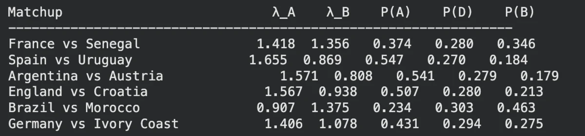
Note: While trying to make the model, I realized that in this particular situation, the Dixon-Coles model is probably not the best way to predict games, considering the lack of xG and xGA data for many teams, quality of opponents during the run-in to the World Cup can drastically vary for different teams due to factors such as region, confederation, opponents resting players, etc. This model is much more suited in a league environment (Premier League/LaLiga). I just wrote about it here cuz it felt interesting enough to talk about. I ended up using the average of actual goals scored and conceded, which again leads to heavy bias towards teams who have only played weaker opponents.
Simulating the Tournament
While individual match predictions are useful, the World Cup is a tournament. You can be the strongest side in the tournament and end up with an early exit just by being in the wrong side of the bracket. A deterministic prediction can totally miss the randomness aspect that any knockout tournament brings. To account for this, I simulated the tournament 10000 times using Monte-Carlo Simulations.
Monte-Carlo Simulations
The name 'Monte-Carlo' comes from the famous Monte Carlo casino in Monaco (here take a 5s time penalty). This is a broad class of computational algorithms that are based on repeated random sampling for obtaining numerical results. The idea is to use randomness to solve deterministic problems.
The core idea is simple: if you want to know the probability of some outcome, but the system producing that outcome is too complicated to calculate directly, you can instead simulate the system a large number of times, and count how often the outcome occurs. The fraction of simulations in which it occurs is your probability estimate. Run it enough times, and the estimate will converge to the true value. The Monte-Carlo method was developed to solve problems that are hard to analytically deal with, due to too many variables or uncertainty. Such problems become easier to solve if we can just define a probability distribution over the inputs and sample from it repeatedly.
Here, our aim is to define a probability model for each match, and then run the full tournament thousands of times, while sampling from these probabilities. After enough iterations, the distribution of outcomes theoretically tends to reflect the underlying uncertainty of the competition.
The Model
To simulate each match I needed a way to translate team strength into expected goals. Rather than the Dixon-Coles approach above, I used FIFA ranking points as a direct proxy for team quality, because they provide a clean, single number for every team in the tournament, and plugged them into a Poisson model.
For any match between team A and team B, the expected goals are:
$$\lambda_A = \text{BASE} \times e^{\Delta / S} \quad \text{and} \quad \lambda_B = \text{BASE} \times e^{-\Delta / S}$$
where $\Delta = \text{FIFA pts}_A - \text{FIFA pts}_B$, BASE = 1.30 (the historical average goals per team per World Cup group game), and S = 900 (a sensitivity parameter: a 500-point gap (Argentina vs Jordan) means Argentina generates roughly 3x the expected goals of Jordan).
The exponential form keeps things symmetric and well-behaved. A stronger team gets more xG, a weaker team gets less, but nobody bottoms out at zero. As a sanity check, using some fixtures in the Group Stage:
| Match | Δ | λ_A | λ_B |
|---|---|---|---|
| Argentina vs Jordan | +488 | 2.24 | 0.76 |
| Brazil vs Haiti | +472 | 2.20 | 0.77 |
| England vs Panama | +288 | 1.79 | 0.94 |
| Switzerland vs Bosnia | +263 | 1.74 | 0.97 |
| Mexico vs South Korea | +96 | 1.44 | 1.18 |
Minnows don't get zero chances, but heavy favourites are around three times more likely to score. That feels about right.
Each match is then simulated by drawing goals independently from $\text{Poisson}(\lambda_A)$ and $\text{Poisson}(\lambda_B)$. In the group stage, a win is worth 3 points, a draw 1 each, and goal difference is tracked for tiebreakers. In the knockout rounds, if the scores are level after 90 minutes it goes to a 50/50 coin flip for penalties. There is no real data to justify anything more sophisticated for neutral-site World Cup shootouts.
The Results
I ran 50000 simulations of the World Cup. Here are the results:
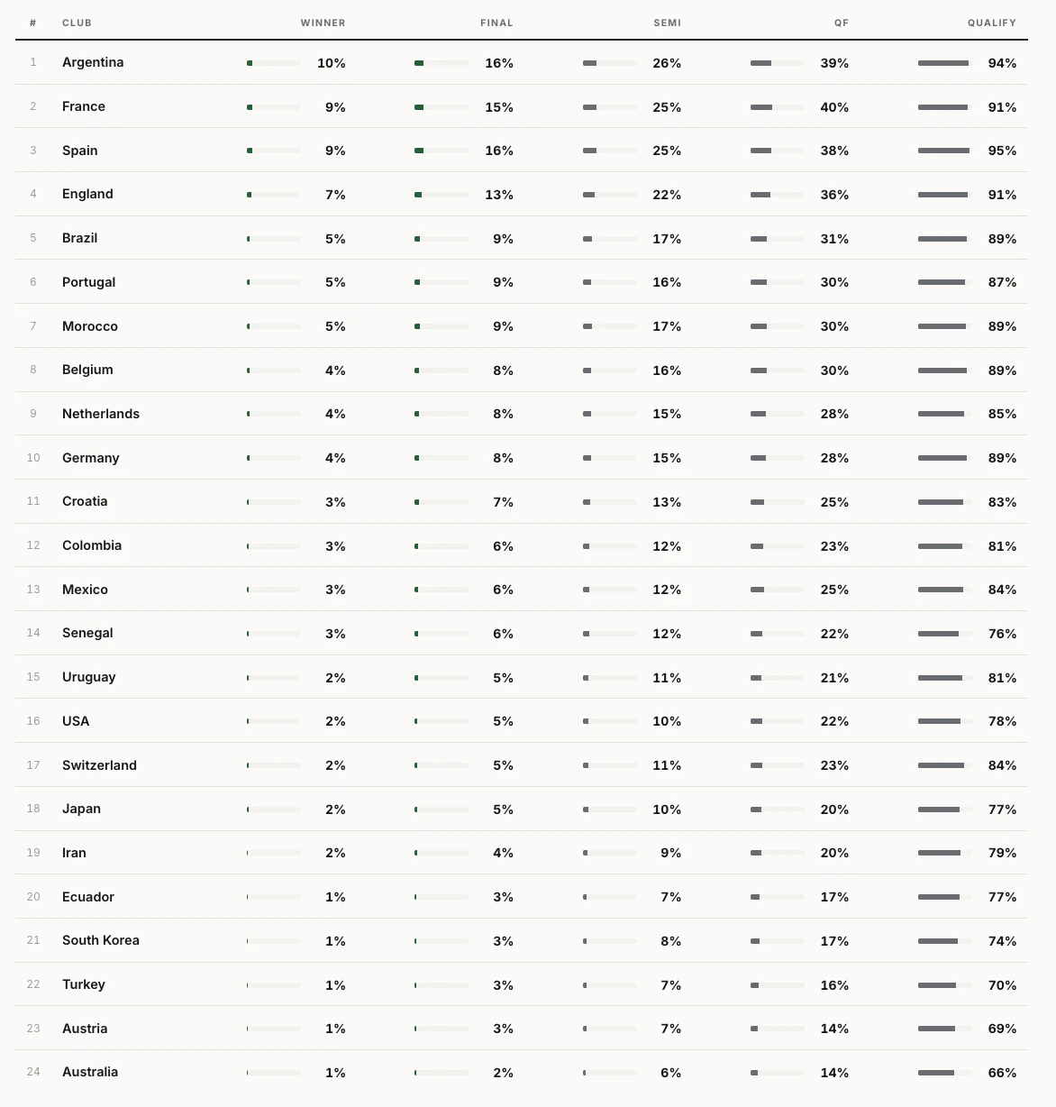
The model has Argentina, France and Spain as the favourites, with the three teams being pretty much neck-and-neck with regard to the chance of winning the tournament. Argentina are ofcourse the defending champiions, having beaten the previous title holders France in a thrilling final in 2022. Spain, the current European champions, are also in the mix with their young and talented squad.
An interesting observation here is how compressed the probabilities are at the top. There is no single 'heavy' favourite while running the simulations before the start of the tournament (can change significantly if I run it after the group stage!), and there are quality teams with a slightly lesser chance (England, Portugal, Morocco) who have had strong performances in recent tournaments and games leading up to the WC.
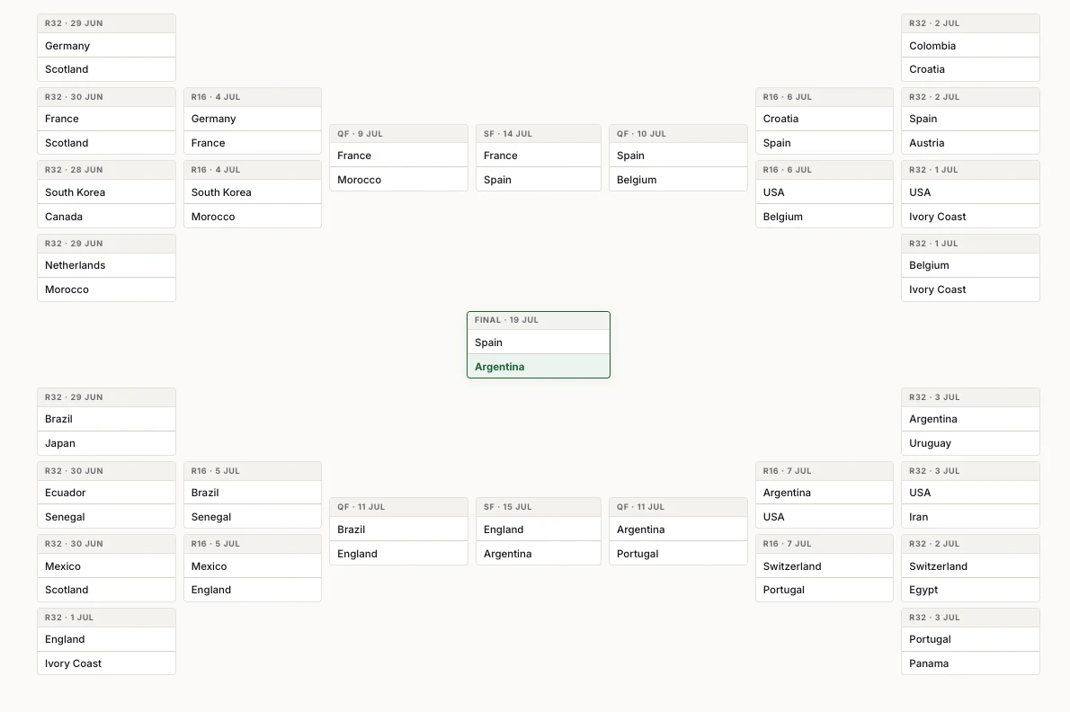
This simulation run is just the most probabilistic representation the 50000 tournaments the model simulated. It is an illustration of how the bracket can unfold when you let the probabilities play out. Things to keep in mind are that it was hard to account for the quality of teams before the tournament (due to lack of free data for multiple teams), and also the fact that knockout tournaments inherently introduce a lot of uncertainty. We have seen shock exits in previous World Cups, and we almost certainly might have a few this year as well.
However, this run does produce a bunch of juicy games, most notably the Argentina vs Portugal Quarter-Final. One last Messi vs Ronaldo showdown, who says no? (Although Messi is clear of CR7 and it's not even a debate). Another good one is the Spain vs Argentina Final, where the best player of the current generation, Lamine Yamal, and the best player of all time, Messi battle it out for the trophy.
Who are you backing this World Cup?